

BitFun Lessons
Water Lesson: River Flood Mapping
Arkansas Flood (Spring, 2019)
In the spring of 2019, the Southern and Central United States have been drenched by rainstorm after rainstorm, leading to widespread flooding. The problem was most acute in late May along the Arkansas River. Every county in Oklahoma was in a state of emergency, and evacuations were ordered or recommended in several communities in Arkansas. In 2019, the continental United States finished its soggiest 12 months in 124 years of modern recordkeeping [ArkansasFlood].
Remote sensing data is widely used in practice to forecast river floods, assess the damage caused, identify flood prone areas, and select places for protective dams to name a few.
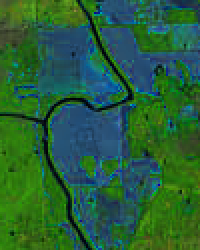
The image below shows flooding near Tulsa, around the suburban town of Bixby, Oklahoma. The image was acquired on May 28, 2019 by Landsat 8 [Landsat8]. For comparison, the same area is shown in May 2018. These are false-color composites, where the colors indicate the following:
- blue - flood waters,
- green - vegetation,
- brown - bare ground.
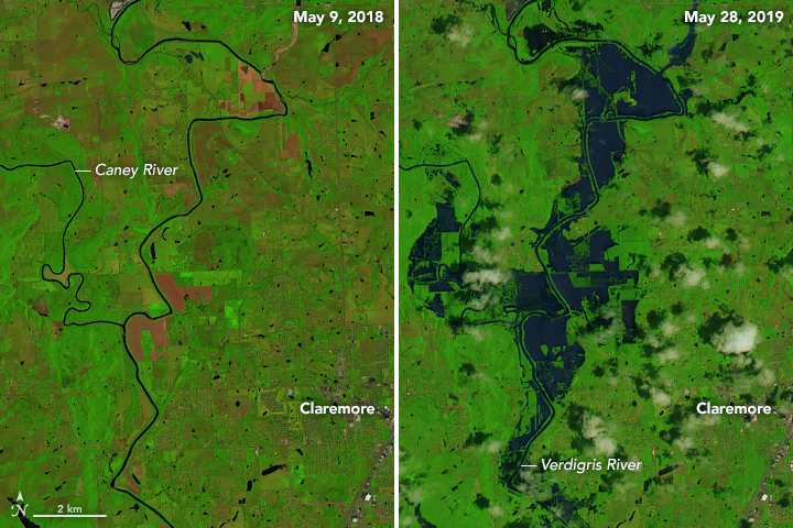
Image source: [ArkansasFlood]
Remote sensing data is much more powerful than building color images. Remote sensing data is used daily for vital tasks including urban planning, agriculture monitoring, forestry control, and rapid-response for disaster relief [ArcGISBook].
We will use remote sensing data for the Landsat 8 satellite to map the flood in the Arkansas River Basin. Landsat Program is the longest continuous space-based record of Earth’s land running from 1972 onwards [Landsat8].
Study Area: Arkansas River Basin
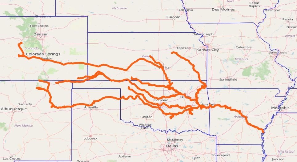
At 1,469 miles (2,364 km), the Arkansas is the sixth longest river in the United States, the second-longest tributary in the Mississippi-Missouri system, and the 45th longest river in the world. The Arkansas generally flows to the east and southeast and traverses the United States states of Colorado, Kansas, Oklahoma, and Arkansas [ArkansasRiver1, ArkansasRiver2]
The Arkansas River drainage basin covers 161,000 square miles (417,000 square km), and has a total fall of 11,400 feet (3,500 m). The average discharge at its mouth is 41,000 ft³/s (1155 m³/s) [ArkansasRiver2].
The image below shows the Arkansas River along with its most noticeable tributaries, U.S. state boundaries, and the city map.
This area serves as a good example, since Arkansas River Basin occupies a relatively large territory over which we must create water masks. BitFun will significantly accelerate mask updates upon the change of the parameter which the mask depends on.
In this example, namely rapid-response/flood mapping, BitFun is especially important as it enables quick re-generation of water masks that depend on a tunable parameter.
NDVI (Normalized Difference Vegetation Index)
NDVI is the most popular index for assessing the state of vegetation and quick land cover classification. In addition, NDVI is used to measure biomass in farming and to quantify forest supply in forestry. Moreover, NDVI is a good indicator of drought [NDVI].
NDVI is calculated as follows:
NDVI = (NIR - RED) / (NIR + RED)
,
where NIR and RED are 2-d arrays with intensities of reflected solar radiation
in the near-infrared and visible red spectra respectively.
NDVI itself is not a tunable function, but if we need to map a flood, we should construct a tunable function that uses NDVI (see below).
River Flood Mapping
To map the flood, we will create a water mask — a 2-d array with two cell values:
1 (water) and 0 (no water).
NDVI values close to zero or negative represent zones with the presence of water.
Hence, to build a water mask, we will evaluate the following inequation:
NDVI - τ < 0,
where τ is a tunable parameter not known in advance, it is usually tuned experimentally.
Mask cells for which this inequation holds, will indicate areas with water. Other mask cells will indicate the absence of water. Note that we use Landsat 8 data, so a cell has an area of about 30 square meters.
BitFun does not read NIR and RED arrays each time the user tunes τ.
This significantly accelerates the computations.
The Goal
As a reference, you will see the RGB map,
resulting mask (recomputed each time you tune τ),
and the set of points of two colors (ground truth) located in flooded and non-flooded areas.
As a User, your goal is to use the visual components of the BitFun Web GUI to tune τ
such that for all ground truth points that indicate flood, the water mask value is 1.
BitFun will re-create the water mask for a large area each time you tune τ,
but this will be almost instantaneous.
References
- [Landsat8] USGS EROS Archive - Landsat Archives - Landsat 8 OLI/TIRS Level-2 Data Products - Surface Reflectance link
- [NDVI] What is NDVI? link
- [ArkansasFlood] Flooding Along the Arkansas River link
- [ArcGISBook] ArcGIS Imagery Book link
- [ArkansasRiver1] Arkansas River link
- [ArkansasRiver2] Arkansas River (New World Encyclopedia) link
Agriculture Lesson: Crop Yield Prediction
Center Pivot Irrigation
Center Pivot Irrigation (or Central Pivot Irrigation) is a method for irrigating crops using sprinklers rotating around a central pivot [PivotIrrigation].
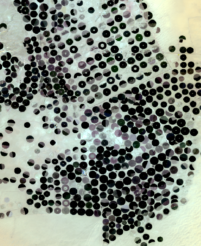
Crop circles can be found in U.S.A., Saudi Arabia, and other countries. This type of irrigation uses less labor (lower costs) compared to other irrigation types and can reduce water runoff, soil erosion, and compaction.
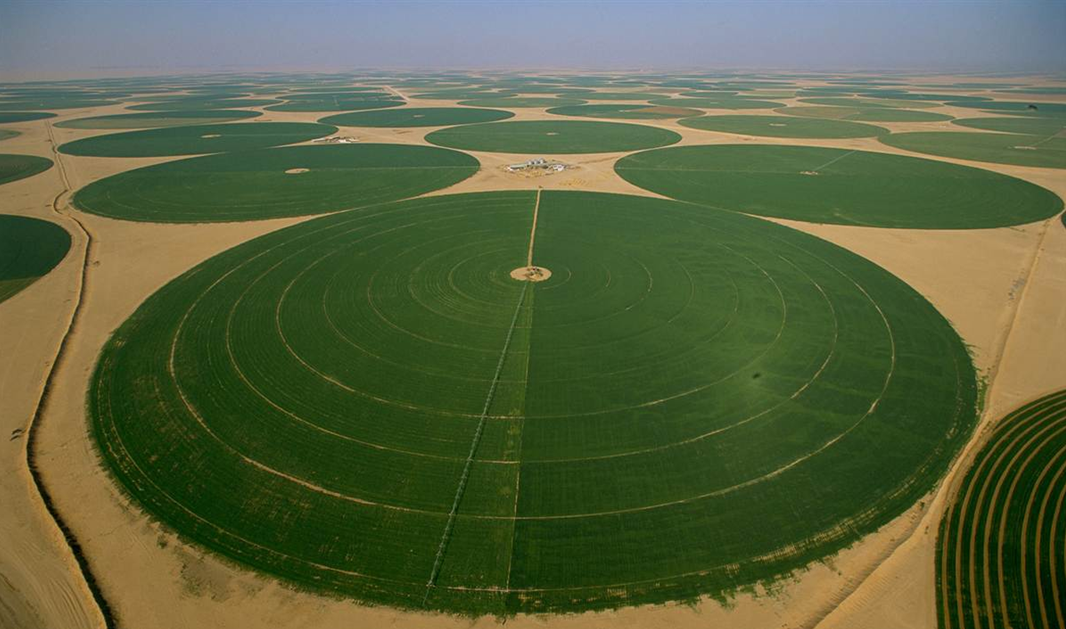
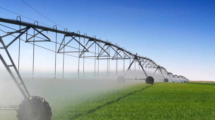
image 1 source, image 2 source
Center pivot irrigation is popular in the arid and hyper-arid regions of the Earth. Fossil water is used for irrigation.
Study Area: Saudi Arabia
In Saudi Arabia, hundreds of fields are irrigated with a number of aquifer wells. The main crops grown in winter are wheat, potato, tomato and melon. Fodder crops, including the biennial multi-cut crops of alfalfa and Rhodes grass, are grown throughout the year [Al-Gaadi2016].
Circles are cultivated in the desert with temperatures reaching 43°C. The water is mined from depths as great as 1 km (3,000 ft). Diameters of fields range from a few hundred meters to as much as 3 km (1.9 mi) [PivotSaudi].
Below is a true-color image of Saudi Arabia center pivot irrigation systems, acquired by Landsat 8 on the 11th of February, 2016 (Wadi Al-Dawasirarea south of Riyadh, the capital city of Saudi Arabia). The image was obtained using Landsat 8 Collection 1 Level 2 data [Landsat8].
We selected this area and time to closely follow the results of [Al-Gaadi2016]. We cannot reproduce the results exactly 1:1 due to at least two reasons: (1) [Al-Gaadi2016] used commercial ENVI software to pre-process the scenes, (2) we do not have the exact parameters for the pivots studied in [Al-Gaadi2016].
Time passed, and Landsat 8 Collection 1 Level 2 emerged which provides already pre-processed Landsat 8 scenes (surface reflectance) [Landsat8]. Hence, we do not use any additional software to pre-process the data as it is no longer required for the purpose of calculating SAVI.
SAVI (Soil-Adjusted Vegetation Index)
SAVI is used for arid regions (such as Saudi Arabia agricultural fields) with sparse vegetation and exposed soil surfaces. SAVI performs much better than other indexes since it aims to minimize soil brightness influence. In contrast, NDVI, another popular index, is very sensitive to soil brightness.
SAVI is calculated as follows:
SAVI = (NIR - RED) / (NIR + RED + L) * (1 + L)
,
where L is a tunable parameter,
a soil fudge factor varying from 0 to 1 depending on the soil.
The value of L is not known in advance and often tuned experimentally.
BitFun provides novel indexing techniques to avoid computing SAVI from
scratch when the user tunes L.
Crop Yield Prediction
We will use the empirical crop yield model for Pivot №44—S for Landsat 8 (Table 4 of [Al-Gaadi2016])
of Saudi Agricultural Development Company (INMA)
in the Wadi Al-Dawasir area south of Riyadh, the capital city of Saudi Arabia:
Yield(t/ha)= 119.79 × SAVI + 11.779
In order to compute Yield, we need SAVI values,
not only classifications as in other cases (e.g. in the water lesson).
Note that we can calculate the Yield up to 2 points after the floating point,
so the BitFun ability to specify precision is very helpful here and will significantly accelerate
computations.
We will feed SAVI values directly to the crop yield model. We will also apply the model to all pivots (i.e., 30 square meters patches), but ideally we should have a separate model for each pivot. If we had many such models, they would be similar. Hence, the number of available models does not influence the BitFun approach.
The Goal
As a User, your goal is to use the visual components of the BitFun Web GUI to tune L
such that the Yield for Pivot №44—S is as close as possible
to the respective value in Table 6 of [Al-Gaadi2016].
BitFun will compute SAVI for a large area each time you tune L.
However, the computations will be lightning fast.
References
- [Al-Gaadi2016] Al-Gaadi et al. Prediction of potato crop yield using precision agriculture techniques. Plos one, 11(9), 2016.
- [Landsat8] USGS EROS Archive - Landsat Archives - Landsat 8 OLI/TIRS Level-2 Data Products - Surface Reflectance link
- [PivotIrrigation] Center pivot irrigation link
- [PivotSaudi] Saudi Arabia Center pivot irrigation link